40. Fractals

Dated: 07-07-2025

Fractal are geometric patterns that is repeated at ever smaller scales to produce irregular shapes and surfaces that can not be represented by classical geometry. Fractals are used in computer modeling of irregular patterns and structure in nature.

According to Webster's Dictionary a fractal is defined as being

"Derived from the Latin word fractus meaning broken, uneven: any of various extremely irregular curves or shapes that repeat themselves at any scale on which they are examined."

Mandelbrot, the discoverer of fractals gives two definitions:

"I coined fractal from the Latin adjective fractus. The corresponding Latin verb frangere means 'to break:' to create irregular fragments. It is therefore sensible - and how appropriate for our needs! - that, in addition to 'fragmented' (as in fraction or refraction), fractus should also mean 'irregular,' both meanings being preserved in fragment"

Every set¹ with a non-integer (Hausdorff-Besicovitch) dimension (D) is a fractal. However not every fractal has an integer \(D\). A fractal is by definition a set¹ for which \(D\) strictly exceeds the topological dimension (D^).

Hausdorff Besicovitch (Fractal dimension)

First, we need to understand the fractal dimension. So first we have to develop an understanding of “how to calculate the dimension of an object”.

Imagine the 3 different objects:

Dividing the line² into \(\frac 1 4\). The idea is self similarity.

Dividing the square into \(\frac 1 4\).

Dividing the cube into \(\frac 1 4\).

If we pay attention to the pattern common in all three, we immediately see that

\[4 = 4^1\]

\[16 = 4^2\]

\[64 = 4^3\]

This gives us equation

\[N = S^D\]

Here \(N\) is the total number of smaller pieces, \(S\) is the scale of 1 small piece compared to larger piece and \(D\) is called the dimension.

\[\implies D = \frac {\log N} {\log S}\]

This dimension is the Hausdorff Besicovitch dimension.

Koch Curve

An equilateral triangle with total length of curve being \(3\).

Length is now \(4\) .

Continue this process and eventually we will get something like

Snowflake fractal

Snowflake for reference

Self Similarity

Barnsley fern example in nature

Fractal Geometry

• For 1 dimensional object (a point on a light), we just need 1 value to describe it.
• For 2 dimensional object (a point on a plane), we need 2 values to describe it.
• For 3 dimensional object (a point in a space), we need 3 values to describe it.

Another mathematical way to define a dimension is to look at how size of an object increases in relation to increase in 1 dimension. Let \(x\) be length in one dimension and \(2\) be the linear scale.

• For one dimension, \(x \implies (2 \times x) \implies 2x\)
• For two dimensions, \(x \times x \implies (2 \times x) \times (2 \times x) = 4x^2\)
• For two dimensions, \(x \times x \times x \implies (2 \times x) \times (2 \times x) \times (2 \times x) = 8x^3\)

So, in general terms

\[S = L^D\]

Where \(S\) is the size, \(D\) is the dimension and \(L\) is the linear scaling factor.

\[\implies D = \frac{\log S}{\log L}\]

In the examples above the value of \(D\) is an integer, \(1, 2\) or \(3\), depending on the dimension of the geometry. This relationship holds for all Euclidean shapes.

Fractal	Euclidean
modern invention	traditional
no specific size or scale	based on a characteristic size or scale
appropriate for geometry in nature	suits description of man made objects
described by an algorithm	described by a usually simple formula

L Systems

The following is based on L Systems as described in "Lecture Notes in Biomathematics" by Przemyslaw Prusinkiewcz and James Hanan.
A brief description of an L system will be presented here but for a more complete description the user should consult the literature.

Simpleminded Example of L System

A string of characters (symbols) is rewritten on each iteration according to some replacement rules. Consider an initial string (axiom)

\[F + F + F + F\]

and a rewriting rule

\[F \to F + F - F - F F + F + F - F\]

After the first iteration, we have

F + F - F - F F + F + F - F + F + F - F - F F + F + F - F + F + F - F - F F + F + F - F + F + F - F - F F + F + F - F

After the second iteration, we have

F + F - F - F F + F + F - F + F + F - F - F F + F + F - F - F + F - F - F F + F + F - F - F + F - F - F F + F + F - F F + F F - F F + F + F - F + F + F - F - F F + F + F - F +  F + F - F - F F + F + F - F - F + F - F - F F + F + F - F + F + F - F F F + F + F - F + F + F - F - F F + F + F - F - F + F - F - F F + F + F - F - F + F - F - F F + F + F - F F + F - F - F F + F + F - F + F + F - F - F F + F + F - F + F + F - F - F F + F + F - F - F + F - F - F F + F + F - F + F + F - F - F F + F + F F + F + F - F - F F + F + F - F - F + F - F - F F + F + F - F - F + F - F - F F + F + F - F F + F - F - F F + F + F - F + F + F - F - F F + F + F - F + F + F - F - F F + F + F - F - F + F - F - F F + F + F - F + F + F - F - F F + F + F - F + F + F - F F F + F + F - F - F + F - F - F F + F + F - F - F + F - F - F F + F + F - F F + F - F - F F + F + F - F + F + F - F - F F + F + F - F + F + F - F - F F + F + F - F - F + F - F - F F + F + F - F 

The graphical meaning for this is

• F means move forward
• + means turn right
• - means turn left

5 iterations
Source: l-systems.netlify.app/

Character	Meaning
F	Move forward by line length drawing a line
f	Move forward by line length without drawing a line
+	Turn left by turning angle
-	Turn right by turning angle
\| (pipe)	Reverse direction (i.e., turn by 180 degrees)
[	Push current drawing state onto stack
]	Pop current drawing state from the stack
#	Increment the line width by line width increment
!	Decrement the line width by line width increment
@	Draw a dot with line width radius
{	Open a polygon
}	Close a polygon and fill it with fill colour
>	Multiply the line length by the line length scale factor
<	Divide the line length by the line length scale factor
&	Swap the meaning of + and -
(	Decrement turning angle by turning angle increment
)	Increment turning angle by turning angle increment

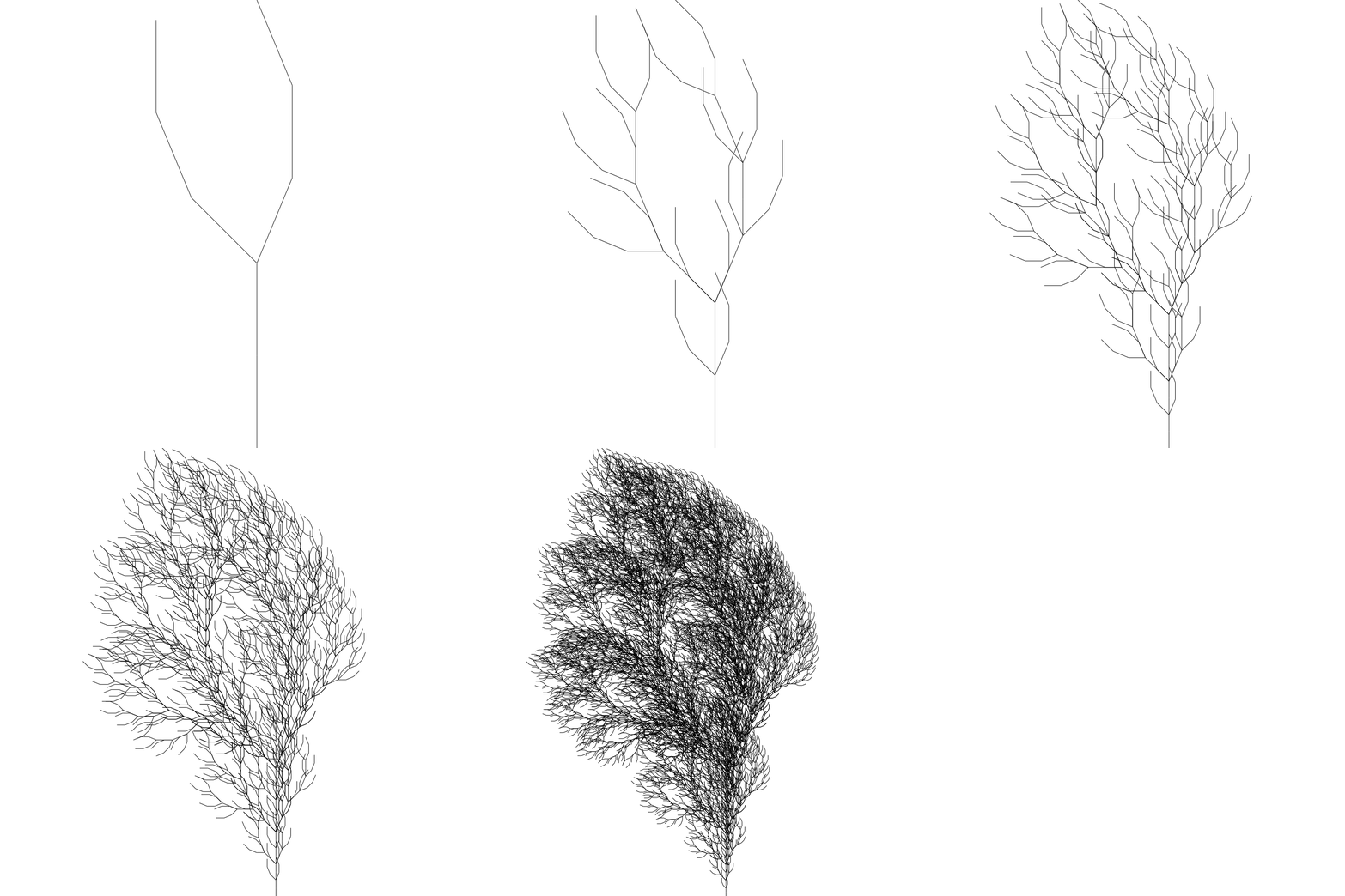
Bush

Axiom

\[F\]

Production Rules

\[F \to FF+[+F-F-F]-[-F+F+F]\]

Turning Angle

\[\theta = 22.5\]

Result

5 iterations
Source: l-systems.netlify.app/

IFS - Iterated Function Systems

Instead of working with lines as in L systems, IFS replaces polygons by other polygons as described by a generator. On every iteration each polygon is replaced by a suitably scaled, rotated, and translated version of the polygons in the generator.

\[ \begin{bmatrix} x_n \\ y_n \end{bmatrix} = \begin{bmatrix} a & b \\ c & d \\ \end{bmatrix} \begin{bmatrix} x_{n - 1} \\ y_{n - 1} \end{bmatrix} + \begin{bmatrix} e \\ f \end{bmatrix} \]

To run the system an initial point is chosen and on each iteration one of the transformation is chosen randomly according to the assigned probabilities, the resulting points \((x_n, y_n)\) are drawn on the page.
As in the case of L systems, if the IFS code for a desired image can be determined (by something called the Collage theorem) then large data compression ratios can be achieved.
The fundamental iterative process involves replacing rectangles with a series of rectangles called the generator. The rectangles are replaced by a suitably scaled, translated, and rotated version of the generator.

Hop along or "The Chaos Game"

\[x_{n + 1} \leftarrow f(x_n, y_n)\]

\[y_{n + 1} \leftarrow f(x_n, y_n)\]

References

---

1. Read more about sets. ↩↩

2. Read more about line. ↩